Understanding MCS Index: The “Speed Limit” of Your Wireless Link
Before you can determine if a slow network is caused by the wireless medium or a TCP session issue, you have to understand the MCS (Modulation and Coding Scheme) Index. Think of the MCS Index as the “negotiated speed limit” between a client and the Access Point.
What is the MCS Index?
The MCS Index is a simple number that represents a complex combination of three factors:
Modulation: How much data is packed into each radio signal (e.g., BPSK, QAM).
Coding Rate: How much of that data is actual payload vs. error correction.
Spatial Streams: How many antennas/radios are being used simultaneously (e.g., 1×1, 2×2, 4×4).
How to Read the MCS Table
When you look at a client’s connection on a Catalyst 9800 or a site survey tool, you will see a value like m9 ss2 (TxRateSet). Here is what that actually tells you:
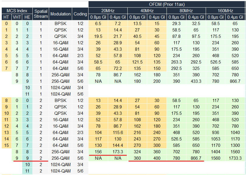
m9 (MCS 9): This indicates the client is using 256-QAM modulation with a 5/6 coding rate. This is a very “dense” and fast signal, but it requires a very clean environment (high SNR).
ss2 (Spatial Streams): This means the client is using two antennas to send and receive data. While some high-end laptops or gaming rigs support 3 or 4 streams, most modern mobile devices are 2×2.
Calculating Your Theoretical vs. Real-World Speed
The MCS Index gives you the Physical Layer (PHY) Rate, which is the maximum theoretical speed. However, wireless is a shared medium with overhead.
The 40MHz Channel Example:
In the scenario shown in the image, a client with m9 ss2 on a 40MHz channel has a theoretical PHY rate of 400 Mbps (using a 0.4μs Guard Interval).
Rule of Thumb: The 0.65 Multiplier Wireless is “half-duplex” and has significant management overhead. To find your expected real-world data throughput, multiply your Data Rate by 0.65.
400 Mbps (PHY Rate)×0.65=260 Mbps (Expected Throughput)
Why This Matters for Troubleshooting
If you run an iPerf test with a single client on the same channel and see only 50 Mbps—despite a solid m9 ss2 (400 Mbps PHY) connection—you can conclude the “Air Interface” is performing well. Since the physical link is healthy, the bottleneck exists further down the line. The culprit is likely a restricted TCP window size, a saturated uplink, or congestion within the core network.
Conversely, if your iPerf is slow and your MCS Index is jumping between m1 and m3, the problem is definitely the wireless medium (interference, low signal, or high noise).
The “Shared Medium” Headache: Managing Multiple Clients
Even if a client has a perfect MCS 9 connection, they are still at the mercy of every other device on the same channel. Because Wi-Fi is a half-duplex medium, only one device (either the AP or a single client) can talk at a time. When you add multiple users to the mix, that theoretical bandwidth starts to divide—often unevenly.
1. The Math of Sharing
If we take our previous example—a 250 Mbps real-world throughput on a 40MHz channel—and introduce a second client, that bandwidth is now shared. If both are actively downloading, your individual speed will drop to roughly 120–130 Mbps.
Note: Low speed results in an iPerf test aren’t always a “problem.” Always check the AP statistics first. If the AP is already pushing 200 Mbps to other clients, your 50 Mbps test is actually a sign of a healthy, saturated channel, not a broken network.
2. The “Slow Client” Penalty
This is the silent killer of wireless performance. In a shared medium, time is more important than speed. A client with a poor RSSI/SNR or an older “legacy” device communicates at a lower MCS index.
The Faster Client: Needs 1ms to send a 100MB file.
The Slower Client: Needs 10ms to send that same 100MB file.
Because the slow client takes 10x longer to clear the air, the fast client is stuck waiting. In high-density environments, one device with a “bad connection” can drag the average speed of every other client down significantly.
3. Optimizing for High Density
To maintain high speeds, you must “groom” your wireless environment to ensure only healthy clients are connected:
Mandatory Data Rates: Disable low data rates (like 1, 2, 5.5, and 11 Mbps). Setting a minimum data rate of 12 or 18 Mbps (and keeping 24+ as supported) forces sticky clients to roam to a closer AP sooner.
RX SOP (Receiver Sensitivity Threshold): Adjusting RX SOP (typically between -75 to -80 dBm) helps the AP ignore “noise” from distant clients, keeping the air clear for those who can actually benefit from high MCS rates.
[redirect to AP channel utilization TS]
The iPerf Playbook: Validating Throughput Like a Pro
When a user complains about slowness, your goal is to isolate the problem. Is it the Wi-Fi signal, the AP saturation, or the TCP stack configuration? Before you even touch iPerf, you must verify the environment.
Phase 1: The Pre-Test Sanity Check
Don’t start a test if the “air” is already broken. Check these three things on your WLC or Dashboard:
Channel Utilization: If it’s above 50%, your results will be low because the medium is already busy.
Client Count: An AP with 15–20+ active clients will show significantly lower per-client throughput.
Physical Link (MCS): Ensure the client is at least M8 or M9 with an SNR above 20dB. If the client is at M4, iPerf will be slow simply because the radio link is weak.
Phase 2: Choosing Your Testing Scenario
The placement of your iPerf server determines which segment of the network you are actually measuring. To find a bottleneck, you should ideally run all three tests and compare the results.
Scenario A (Client & Server on the same AP): Tests the “Air-to-Air” performance.
Note: Expect your throughput to be cut by roughly 50% here, as the AP must receive and then re-transmit every packet on the same half-duplex channel.
Scenario B (Same SSID, Different APs): Tests the wireless medium quality plus the infrastructure between APs.
If using Centralized Switching, this tests the path from AP1 to the WLC and back to AP2.
If using FlexConnect on the same switch, it tests the local Layer 2 switching performance between APs.
Scenario C (The Gold Standard): Server on the wired network (same VLAN/SVI), client on wireless.
This is the best way to test the Wireless-to-Wired handoff. It isolates the Wi-Fi link from any wireless-to-wireless overhead, giving you the clearest picture of the client’s actual capability.
Why Comparative iPerf Testing is Essential:
Running a single iPerf test only tells you that the network is slow; running all three tells you why. Comparing these scenarios side-by-side is the only way to definitively pinpoint whether the lag is a wireless medium issue or a wired infrastructure problem.
Scenario 1: The Infrastructure/Tunnel Bottleneck
The Result: Scenario A is fast, but B and C are significantly slower.
The Conclusion: The “Air Interface” is healthy, but the issue lies in the transport.
Centralized Switching: There is likely congestion or a bottleneck within the CAPWAP tunnel or the physical link between the APs and the WLC.
FlexConnect: The bottleneck is likely in the switching fabric between the two APs.
Scenario 2: The Wired Network Bottleneck
The Result: Scenarios A and B are fast, but C (Wireless-to-Wired) is slow.
The Conclusion: The entire wireless ecosystem—including the air, the APs, and the CAPWAP tunnels—is performing perfectly.
The issue is located beyond the wireless handoff. You should investigate the distribution/core switches, the wired infrastructure, or the server’s own network stack. This proves the issue is not on the wireless side.
Phase 3: Executing iPerf3 Commands
Navigate to your iPerf3 folder in CMD/Terminal and set up your endpoints.
The Basics:
Server Side:
iperf3 -sClient Side:
iperf3 -c <server-IP>
Phase 4: Pro-Level Tuning (TCP vs. UDP)
Standard TCP tests often fail to reach max speeds due to “Window Size” limitations or latency. To see what the network is actually capable of, use these advanced flags:
TCP Window Size (-w)
If you have latency, the “window” fills up and the sender waits for ACKs, slowing the test. Match your window to your expected speed:
150–600 Mbps: Use
-w 250k200 Mbps – 1.2 Gbps: Use
-w 500kHigh Speed / Low Latency: Use
-w 2m
Parallel Streams (-P)
Running a single stream might not saturate the link. Use -P 2 or -P 4 to send multiple streams at once. Note: Your total result is the sum of all streams.
UDP Testing (-u)
TCP has too much overhead for some tests. To see the raw “brute force” capacity of the link, use UDP:
iperf3 -c <SERVER_IP> -u -b 700MThis pushes a constant 700 Mbps stream to see where the “breaking point” of the packet loss begins.
Summary: The “Best Practice” Command
For a comprehensive wireless test that accounts for latency and saturates the link, run this: iperf3 -c <SERVER_IP> -w 500k -t 20s -i 1s
Pro-Tip: Always Test Both Directions
Wireless traffic is often asymmetrical—your download speed might be excellent while your upload struggles (or vice-versa). To get the full picture, you must test both directions:
Standard Test (
iperf3 -c <server>): The client uploads data to the server.Reverse Test (
iperf3 -c <server> -R): The server sends data to the client (testing the client’s download speed).Mobile devices and laptops often have smaller antennas and lower transmit power than an Access Point, so running the
-Rflag is the only way to see if a bottleneck is specific to the client’s ability to push data back to the network.
The Math Behind the Speed: The TCP Throughput Formula
Even if your wireless link is perfect, your actual data speed is governed by the TCP Receive Window (RWIN) and the Round Trip Time (RTT). If the window is too small or the latency is too high, the sender spends more time waiting for acknowledgments (ACKs) than actually sending data.
The Formula
To calculate the maximum theoretical TCP throughput, use this equation:
TCP Throughput (bps) = Window Size (bits) / RTT (seconds)
Breaking Down the Variables
Window Size: This is the amount of data a receiver is willing to accept before sending an ACK. In iPerf3, you adjust this with the
-wflag.Note: Remember to convert Bytes to Bits (multiply by 8).
RTT (Round Trip Time): The time it takes for a packet to go to the destination and for the ACK to return.
Note: Convert milliseconds to seconds (divide by 1,000).
Real-World Example
Let’s say you are running an iPerf test with a 500 KB window and your ping (RTT) is 40ms.
Window Size in bits: 500,000 Bytes×8=4,000,000 bits
RTT in seconds: 40ms/1,000=0.040 seconds
The Calculation:
Window Size in bits: 500,000 Bytes × 8 = 4,000,000 bits
RTT in seconds: 40ms / 1,000 = 0.040 seconds
Result: 4,000,000 / 0.040 = 100,000,000 bps (100 Mbps)
⚡ Pro-Tip: Skip the Manual Math
While it’s important to understand how the window size and latency interact, you don’t have to do the heavy lifting yourself every time you’re troubleshooting on-site.
For a quick and accurate calculation of your theoretical limits, I recommend using this Online TCP Throughput Calculator:
Why This Matters for Wireless Troubleshooting
If your iPerf test is capping out at 100 Mbps, but your wireless MCS Index says you should be hitting 400 Mbps, look at your latency!
A high RTT (Round Trip Time) acts as a bottleneck, but it doesn’t tell you why the delay is happening. The lag could be caused by wireless interference, a layer 2 loop, random packet drops, or even a server that is slow to respond.
Regardless of the cause, a standard TCP window will “throttle” your speed to wait for acknowledgments. To bypass this “math wall” and see the true raw capacity of your network path, you must manually increase the window size in your iPerf3 test (e.g., -w 2m).
The Takeaway: A “slow” iPerf result doesn’t always mean a “slow” network. It might just be an “unoptimized” TCP session for that specific link’s latency.
Deep Dive: Analyzing a Slow TCP Connection in Wireshark
When iPerf results come back lower than expected, we need to look at the packet level to see how the TCP stack is behaving.
1. The Acknowledgement Gap
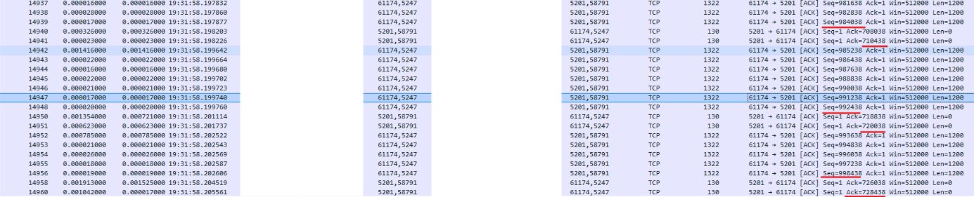
Initially, the client transmits approximately 11,000 bytes of data (multiple segments sent in a single burst). However, looking at the server’s response, it only acknowledges 7,000 bytes.

The server is already falling behind. The client is pushing data faster than the server can process or the network can deliver the acknowledgments.
2. The Widening Discrepancy
In the subsequent packets, the client continues its pace, sending an additional 14,000 bytes (totaling 25,000 bytes sent). The server remains overwhelmed, acknowledging only 12,000 bytes.

This confirms the server/network path is struggling. Server is falling behind by 13,000 bytes and was only able to catch up by a measly 5,000 bytes, proving the bottleneck is consistent.
3. The Critical Breaking Point
The situation reaches a critical state at the 1 million byte mark. The client has pushed significantly more data than the server can acknowledge (270,000 bytes).
Using the Throughput Graph to Pinpoint the “Sweet Spot”
If we investigate the Wireshark throughput graph for this session, a clear pattern emerges. Once the client reaches a certain volume of data (around 1 million bytes), the throughput drops significantly.
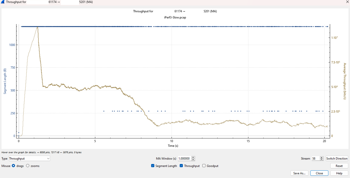
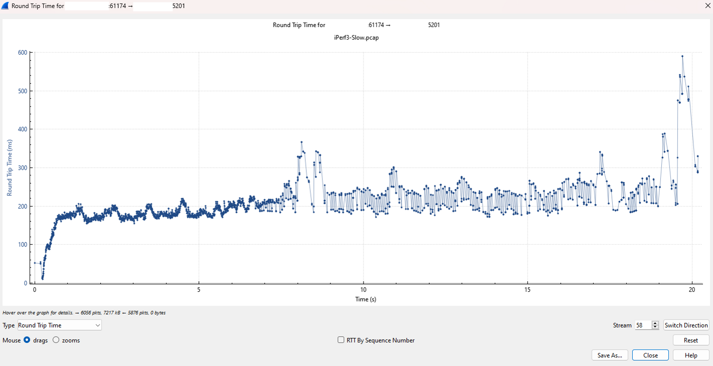
This decline happens because the protocol is searching for a “sweet spot”—the maximum speed at which the server can actually keep up with the incoming ACK sequence IDs without dropping data. When you see this drop, it suggests one of two things:
Network Congestion & Path Saturation: By analyzing the RTT (Round Trip Time) graph, we can see latency spikes that far exceed the baseline for a healthy link. This visual confirmation proves the network path is saturated, meaning the “pipes” are full and packets are being delayed as they wait in queue.
Server Overload: The server’s buffer is full, and it cannot “unload” or process the data fast enough to send timely acknowledgments.
Why iPerf is the “Cleanest” Test
The beauty of using an iPerf test for this analysis is that it virtually eliminates the risk of server-side application lag. Because iPerf is a “dummy” application—designed specifically to send and acknowledge data without actually processing it—a slow result almost always points to the network latency or packet drops at a specific hop, rather than a slow server (App issue).
Deep Dive: Analyzing a Healthy TCP Connection in Wireshark
When network performance is optimal, Wireshark provides a roadmap of how efficient communication should look. By examining the packet level, we can see exactly how the TCP stack manages fragmentation and maintains synchronization.
1. Handling the CAPWAP MTU Constraint
In this capture, the client begins transmitting data without a defined TCP MSS “headcap.” Consequently, TCP attempts to squeeze through 1460 bytes—the maximum size possible for a standard Ethernet frame. However, because this traffic is traversing a CAPWAP tunnel, it encounters additional overhead that lowers the available MTU.
To compensate for this “tight fit,” the stack is forced to fragment the data into two pieces:



Fragment 1: 1485 bytes
Fragment 2: 52 bytes
Despite this fragmentation, the flow remains seamless, ensuring the data fits within the tunnel’s maximum MTU limits without causing drops.
2. Maintaining the Synchronization Pace
Unlike a struggling connection, the “Acknowledgement Gap” here is virtually non-existent. The session starts with a transmission of approximately 14,000 bytes, and the server responds by acknowledging that exact amount almost instantaneously.
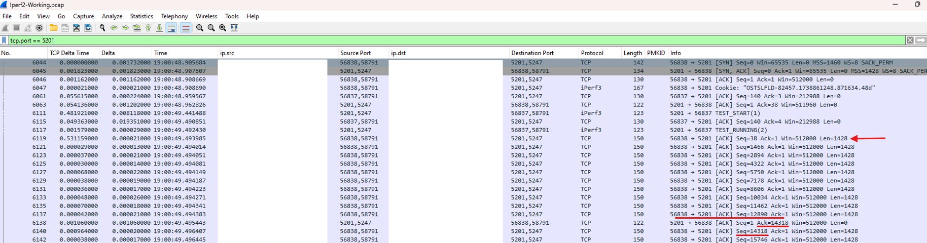
As we progress through the capture, the server maintains a perfect pace with the client. Every burst of data sent is met with a corresponding ACK, resulting in a minimal discrepancy by the end of the stream. This confirms that the server and the network path are operating in perfect harmony.




3. Verification through Throughput and RTT
To validate the health of this session, we look at the stability of the transfer over time.
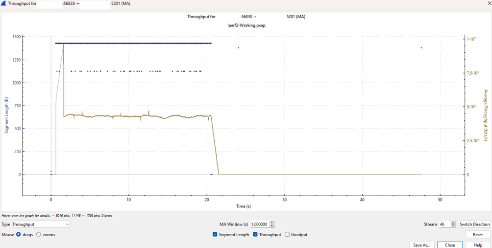
Consistent Throughput
The throughput graph shows a rock-solid, flat line during the transmission phase. There are no sudden collapses or “searching” for a stable rate; the protocol finds its maximum speed immediately and holds it until the transfer is complete.
Healthy Latency (RTT)
The Round Trip Time (RTT) graph provides the final piece of the puzzle. We see a consistent baseline of latency, with the majority of packets being acknowledged within 5 to 20 milliseconds.
While there are occasional jitter spikes peaking at 45ms, they are transient and do not disrupt the overall flow. This indicates a stable link where the “pipes” are appropriately sized for the traffic volume.
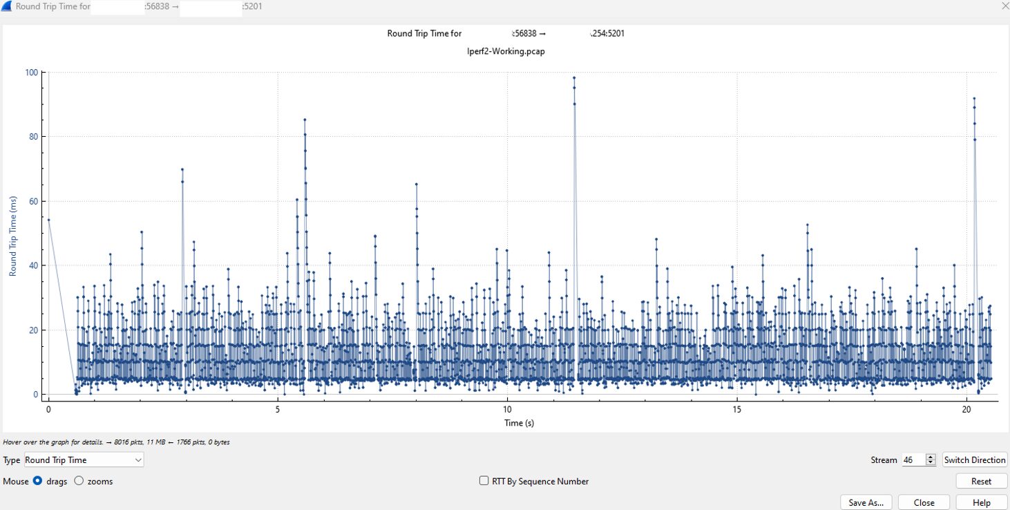
Summary Verdict: This capture represents an ideal “Working” scenario. Even with the added complexity of CAPWAP encapsulation, the TCP stack remains efficient, providing high throughput with predictable latency.
Further Reading & Resources
To expand your understanding of TCP mechanics and flow analysis, I highly recommend exploring Chris Greer’s blog and YouTube channel, where he breaks down complex packet events with incredible detail. For a technical deep dive into identifying packet loss and sequence issues, check out this comprehensive Wireshark TCP Trace Graph Tutorial and his guide on How TCP Works.